How solar irradiance, shading, and string design are calculated in solar PV

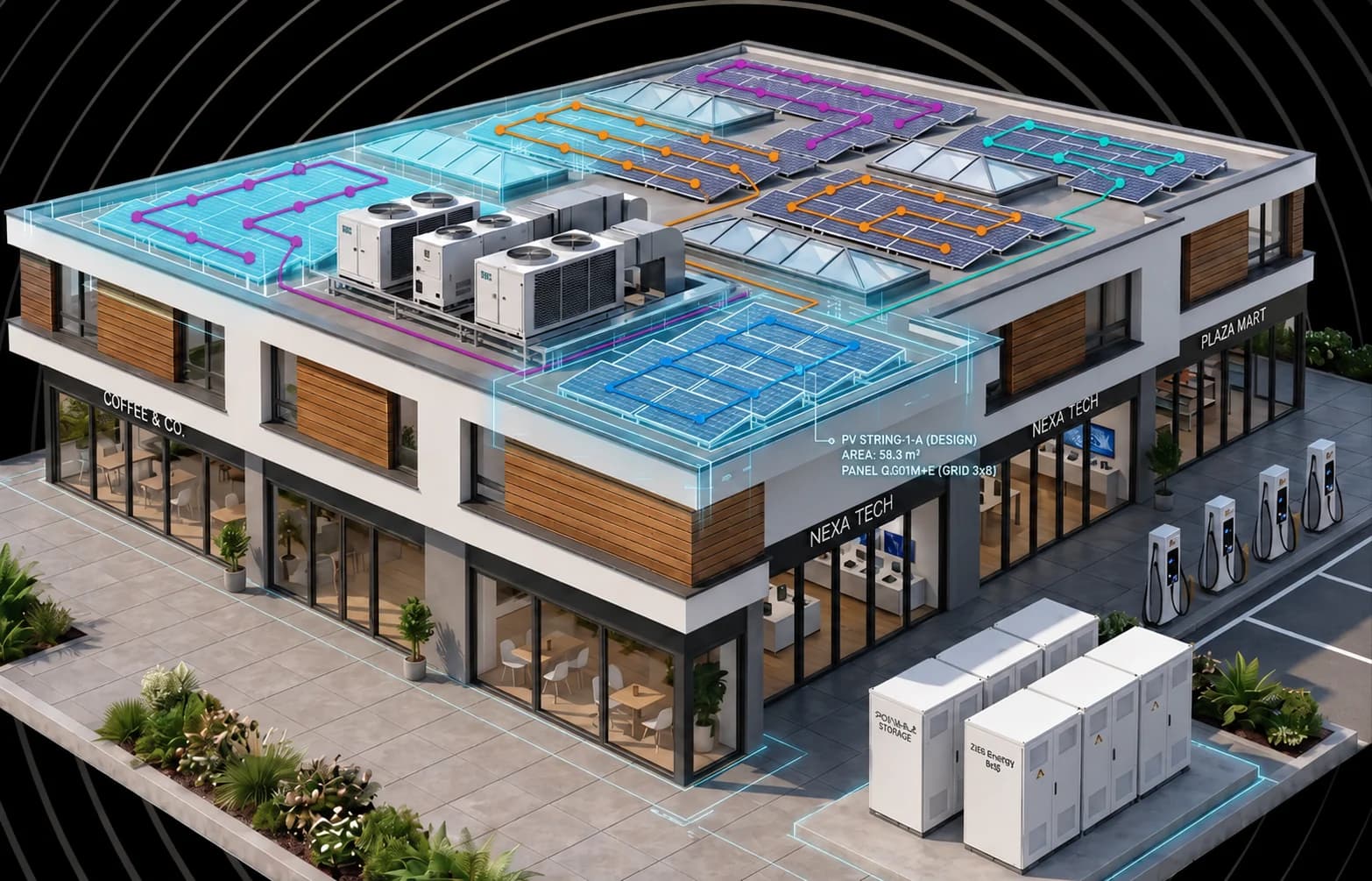
Every solar production estimate rests on two calculations that most software hides behind a single number: how much sunlight actually reaches each panel, and how those panels behave once they are wired into strings and connected to an inverter. Get either one wrong and the yield figure on the proposal is fiction. This guide walks through how solarVis performs both, the irradiance and shading model on the optical side, and the string and inverter model on the electrical side, so that installers, designers, and engineers can see exactly what sits behind the production number.

What is solar irradiance?

Solar irradiance is the amount of solar energy received per unit area as electromagnetic radiation, typically measured in kWh/m²/year. It is the raw resource that a photovoltaic system converts into electricity, and it is never a single quantity arriving from a single direction. It reaches a surface as three distinct components.

Direct, diffuse, and reflected irradiance

Direct irradiance (beam irradiance, or DNI, Direct Normal Irradiance) travels in a straight line from the sun to a surface without being scattered. It is the most intense component and dominates under clear-sky conditions.

Diffuse irradiance (DHI, Diffuse Horizontal Irradiance) has been scattered by molecules, aerosols, and clouds in the atmosphere before reaching the surface. It arrives from all directions of the sky and becomes dominant under cloudy conditions.

Reflected irradiance (ground-reflected, or albedo irradiance) is radiation that reflects off surrounding surfaces such as the ground, buildings, or other objects before reaching the surface of interest.

The final irradiance on a panel is obtained by combining all three components. Separating them is not academic: each one interacts with shading differently, which is why they have to be modeled separately before being summed. The decomposition of global irradiance into beam and diffuse components follows the same physics used across the solar engineering literature^[5][4].

How solarVis calculates shading and irradiance

SolarVis derives irradiance for a project's roof by aggregating weather data from multiple sources for the exact project location, then processing the three components against the 3D model of the site. Direct and diffuse radiation are handled with two different geometric methods.

Direct irradiance: cell-level ray tracing

For the direct component, shading is evaluated with a ray-tracing approach. Each cell on the panel surface is treated as a point from which a ray is cast toward the sun. If the ray reaches the sun unobstructed, the point is unshaded; if an obstacle intercepts it, the point is shaded.

This test is repeated for every time step across the year at hourly resolution. Each point is assigned a binary value at each step, 1 when the ray reaches the sun and 0 when it is blocked. Aggregating these results over time yields the effective direct irradiance actually landing on the panel, rather than a flat percentage guess.

Diffuse and reflected irradiance: hemispherical visibility

Diffuse and reflected radiation arrive from the whole sky dome, not a single point, so they need a different treatment. For each point on the panel, rays are cast outward across the hemisphere to measure how much of the sky and surrounding environment is visible. Instead of a time-based trace toward the sun, this is a spatial analysis of the sky dome.

The result is a percentage representing the accessible share of diffuse and reflected radiation. That percentage is multiplied by the corresponding diffuse and reflected irradiance values from the weather data to produce the final component values. Summing direct, diffuse, and reflected gives the total irradiance for that point.

Solar access, TOF, and TSRF explained

Three derived metrics translate raw irradiance into a language you can use to compare roof faces and panels. They appear in the solarVis inspector as you hover over the model, and they are worth defining precisely because they are frequently confused.

What is solar access?

Solar access is the percentage of solar radiation that reaches a surface after shading is taken into account. It measures how much of the available sunlight is not obstructed by surrounding objects.

Solar access = irradiance received with shading ÷ irradiance received with no shading

For example, a solar access value of 96 percent means that 4 percent of the potential solar radiation is lost to shading.

What is TOF (Tilt and Orientation Factor)?

TOF, the Tilt and Orientation Factor, is expressed as a percentage and compares the solar insolation at a panel's actual tilt and orientation to the maximum possible insolation at the optimal tilt and orientation. It is calculated separately for each roof face, because each face has its own slope and azimuth. TOF isolates the geometric penalty of a roof, independent of shading.

What is TSRF (Total Solar Resource Fraction)?

TSRF, the Total Solar Resource Fraction, combines both effects. It is the ratio of the insolation available at a surface, accounting for shading and TOF, to the insolation at the optimal tilt and orientation with no shading.

TSRF = solar access × TOF

TSRF is the single most useful figure for judging a roof face, because it folds the shading loss and the geometric loss into one number. A steep, poorly oriented roof with no shading and a flawless, heavily shaded roof can produce the same disappointing TSRF for very different reasons, and the metric tells you to keep looking.

What is a string in a solar PV system?

A string is a group of solar panels that are electrically connected in series. Two elements define a string: the panel and the inverter. Everything about string design comes down to keeping the combined electrical output of the series-connected panels inside the operating window of the inverter, across every temperature the site will ever see. To do that accurately, each panel and the inverter both have to be modeled from first principles rather than nameplate ratings.

Modeling the panel: the single-diode model

Each panel is modeled with the single-diode equivalent circuit. In this model, the unknown parameters are derived by solving equations based on the values from the panel datasheet, which lets solarVis generate the I–V and P–V curves of the panel cells under any given irradiance and temperature.

The key parameters, including the series resistance (Rs) and shunt resistance (Rsh), are solved from the characteristic points on the datasheet:

• Open-circuit voltage: V = Voc, I = 0
• Short-circuit current: V = 0, I = Isc
• Maximum power point: V = Vmp, I = Imp

Because Voc, Isc, Vmp, and Imp come straight from the manufacturer's datasheet, fitting the model to these known operating points solves the equivalent-circuit parameters and produces an accurate I–V characteristic under varying conditions. This five-parameter approach is the validated, industry-standard method for single-diode PV modeling^[3][8].

Bypass diodes, half-cut cells, and partial shading

A critical part of panel modeling is the module's internal structure, specifically whether it uses bypass diodes or half-cut cell technology. Modeling these lets solarVis represent panel behavior accurately under partial shading, which is exactly the condition where simplistic derate models fail.

Panels wired in series share the same current, so a single shaded panel would otherwise throttle the whole string. Bypass diodes let current route around a shaded cell group, and half-cut layouts split the module so that shading one half does not penalize the other. By building the string curve from real modeled panel curves, solarVis captures the true, non-linear cost of shade instead of applying a flat percentage.

Modeling the inverter: MPPT voltage and current limits

The inverter is modeled from its Maximum Power Point Tracker (MPPT) characteristics: the operating voltage range and the current limits.

The MPPT voltage range (for example 100 V to 500 V) sets the allowable operating window. This range determines how many panels can be connected in series in a single string, so that the total string voltage stays within the inverter's limits. The inverter's maximum input current (for example 16 A per MPPT) determines how many strings can be connected in parallel, so that the combined current of the parallel strings does not exceed the inverter's capacity. These two constraints define the electrical envelope of the system and feed directly into the production calculation.

String sizing: how many panels in series and parallel

To size a string correctly, panel behavior has to be evaluated at temperature extremes. Using the minimum and maximum ambient temperatures for the location, and the temperature coefficients for Voc and Isc from the datasheet, solarVis adjusts the panel's electrical characteristics for those conditions. This is what keeps a system safe and efficient in both a cold clear morning and a hot afternoon.

Series limits: temperature-corrected Voc

Panel Voc rises as temperature falls, so the coldest moment of the year is when a string is most likely to overshoot the inverter's maximum voltage. That sets the ceiling. The hottest moment sets the floor, because Voc sags and the string can drop below the MPPT minimum.

These limits guarantee that the string voltage stays inside the inverter's operating range in every weather condition, which is exactly what array design standards require designers to verify^[7].

Parallel limits: Isc at maximum temperature

Multiple strings can be connected in parallel on one MPPT input, bounded by the inverter's maximum input current. Panel Isc rises slightly with temperature, so the worst case is the hottest condition.

For example, an inverter with a 100 A maximum input current sets the parallel limit by dividing that figure by the panel Isc under worst-case (maximum temperature) conditions. Together, the series and parallel limits keep both voltage and current inside safe boundaries while feeding accurate numbers into the production model. The temperature-dependent behavior that underpins all of this is defined in the module energy-rating standards^[6].

From strings to production: the MPPT power calculation

Once individual panel curves are defined, system behavior is built up by combining panels into strings and strings into MPPT inputs.

For a series connection, the panels share the same current while their voltages add, so the string I–V curve is obtained by summing the voltage of every panel at each current level, advanced characteristics like half-cut structure and bypass diodes included. For a parallel connection, the voltage is the same across strings while the currents add, so the MPPT I–V curve is derived by summing the current of all connected strings at each voltage level.

Production is then calculated per MPPT. Using the P–V curve, the system finds the maximum power point that lies within the inverter's constraints, its maximum input current and its minimum and maximum MPPT voltage. That point is the highest achievable power under the given conditions. The calculation runs for a single hourly time step and then repeats for every hour using that hour's irradiance and temperature, and aggregating the results over the year gives total energy production.

Why this matters for your proposals

The reason to model all of this rather than approximate it is that the errors compound. A flat shading derate hides which roof face is actually worth using. A nameplate-only string check passes a design that trips the inverter on the coldest morning of the year. A uniform production factor buries the fact that one shaded panel is dragging a whole string. When the physics is modeled properly, the yield figure on the proposal is one you can stand behind, and the loss chart shows the customer exactly where every kilowatt-hour went.

This is the engine behind Solar 3D Design and Simulation, and it flows straight into solar proposal generation, where the shading and stringing losses appear in a transparent loss chart. If you are pairing PV with storage, the same modeled production drives battery modeling. For the full workflow, see the solarVis docs on drawing strings and assigning them to MPPT inputs and on panel placement, shading, and irradiance analysis.

The fastest way to understand the model is to run it on a roof you know. Load a real project, turn on shading analysis, draw a string, and watch the Voc, Vmpp, and Isc validate against the inverter in real time.

References

- European Commission JRC, Photovoltaic Geographical Information System (PVGIS)
- NREL, PVWatts Calculator
- De Soto, Klein & Beckman, Improvement and validation of a model for photovoltaic array performance (Solar Energy, 2006)
- Perez et al., Modeling daylight availability and irradiance components from direct and global irradiance (Solar Energy, 1990)
- Duffie & Beckman, Solar Engineering of Thermal Processes (Wiley)
- IEC 61853, Photovoltaic (PV) module performance testing and energy rating
- IEC 62548, Photovoltaic (PV) arrays, Design requirements
- pvlib python, open-source PV modeling library (Sandia National Laboratories)